Spread the love
First of all, you should understand how 3D processing differs from 2D. 2D toolpaths are used almost exclusively for machining parts that are prismatic, meaning all surfaces of the part are horizontal or vertical.
3D toolpaths are used to process parts with more arbitrary shapes - they may not have perfectly vertical or horizontal surfaces. The image below shows the 3D part on the left and the prismatic part on the right.
Differences between 2D and 3D processing
Roughing and finishing
An important difference between 2D/3D for CAM programs is that 3D machining is often divided into clearly defined roughing and finishing steps. The bulk of the original material is removed by the roughing path as quickly as possible, although this may leave a poor quality surface. Finishing paths are used to remove small amounts of material and give a part the desired surface finish in a minimum amount of time.
2D toolpaths also use roughing and finishing passes, but they are often combined into one operation. For example, a pocket may be cut slightly smaller and then trimmed to its final size on a final pass all the way through.
You want the processing time of your part to be as short as possible, and you also want an accurate model with a smooth surface. When using only one operation, you have to choose between speed or accuracy. Since the cutter cannot remove all the material at once (except on very thin models), it will move down the layers. For example, immersing it 5 mm into the material removes all excess material above this level; next plunge to minus 10, etc. DeskProto will automatically apply this layering (which is the roughing functionality) since it will not allow the cutter to go deeper into the material than the length of the cutting part (at least in the first operation). When this is done in small increments (required for a smooth surface), it takes a lot of time.
When using roughing and finishing: the roughing operation will quickly remove material (using a large tool path spacing), after which the finishing operation will produce an accurate model and smooth surface (using a small spacing).
To do this we need to have two operations in DeskProto, so you need to create a second operation for the current part. You can do this in several ways: as shown above, this is by right-clicking in the tree on the Part line, and then selecting Add Operation from the context menu. The result will be a tree with two operating operations called “Operation” and “Operation [#1]”.
Double-click on the first row of the operation in the tree and change its name to “Roughing”. This concerns the operation you opened in the previous point: in case you have made a lot of changes, you will first be better off in the context menu to switch Operations 1 and 2 with 'Move up' or 'Move down' ). You can now set the operation parameters to make it truly a Roughing Operation. Go to the Roughing tab and select Layer height i.e. the height of the entire layer (the default value is the length of the cutter, which in many cases will be too large) and the thickness of the Skin (the layer removed per pass). For a 6mm router bit and softwood, you can use 10mm layer height and 0.5mm removal layer (in inches: for a 1/4" router bit this is 0.4" layer height and 0.02" removal layer). You can also check the Ramping parameter. Use Help for more information about these settings.
For the roughing strategy (2nd tab), we often use Block because it is the most efficient in most cases. However, not for this frame as this will release the material in the center causing problems. Therefore, keep the Parallel strategy.
The General tab now allows you to select larger precision values (distance and step size). In most cases, the second value in the dropdown list will be: d/3. This means 1/3 of the cutter's diameter, so you'd expect 2mm (0.0833"). Now instead of d/3 it will be reported as 2.33 mm (0.0967″). The reason for this difference is the release layer that was applied. The layer to be removed is processed by calculation using a “virtual cutter”, which is thicker than the real one: R 3 + skin 0.5 = R 3.5. This means that the diameter becomes 7, and the step size of 7.0 / 3.0 results in 2.33. Close the dialog using OK.
The second operation will be Finishing Operation: open the options, and change the name to “Finishing”. You do not need the roughing functions in place and want to reduce the precision values (distance and pitch). For finishing we often check the 'Skip horiz' option. Ambient' i.e. skip the horizon. environment (Advanced tab), also uncheck “ignore enclosed ambient”, which will allow the frame to skip the central hole. This will only shorten the tool path if the Sort option is checked on the Movement tab. You can leave everything else as it was (default values).
You can use two different cutters for roughing and finishing: a thick flat cutter for fast, efficient roughing, and a small ball-tip cutter for finishing detailing. Since this geometry contains many small details, this will give a very good result. On the other hand: the alternative of using the same cutter for both operations has the advantage that there is no need to change tools.
Roughing
In many cases, 3D roughing passes are very similar to pocket paths used in 2D machining. The model is divided into several slices, each of which is machined so that the model remains “inside” the workpiece.
Parallel roughing
The image above shows a parallel roughing path, also called a zigzag path. As with regular 2D pocket cutting toolpaths, you usually have options such as offset toolpaths:
Roughing with offset
The parallel and offset paths shown above are based on standard 2D pocket paths where the Z level is locked for each slice. This leads to a problem where a lot of material is left uncut:
Simulation of flat roughing cutting
We can reduce this significantly if we project each slice onto the model so that the Z level can follow the contours of the part.
Rough 3D processing, side view
When we look at the simulation, we get:
3D Roughing Cutting Simulation
Looking at the result, it may not be immediately clear why you chose the flat version in the first place. Of course, there's one big reason you might prefer a flat path - it will often cut faster because the machine doesn't have to move the Z axis up and down while cutting. The exact difference in speed depends entirely on your model, your machine, and your feed speed.
My rule of thumb is that if I'm cutting a soft material like plastic or foam, where I can use high feed rates without stressing the machine, then I prefer a flat roughing toolpath. Excess stock will not be a problem for the finishing pass, and I like the faster machining time.
However, if I'm cutting a hard material like metal, I prefer the 3D roughing toolpath. Most likely the processing time will be limited by my feed speed and I prefer to leave a small even film for the finishing pass.
After roughing, most of the excess material should be removed from the stock. We can now move on to the finishing toolpaths where the part will be cut to its final dimensions with an acceptable surface finish.
Cutting speed
Very important values that influence cutting conditions during turning are cutting speed (v) and spindle speed (n). In order to calculate the first value, use the formula:
where π is the number Pi equal to 3.12;
D – maximum diameter of the part;
n – spindle rotation speed.
If the latter value remains unchanged, then the rotation speed will be greater, the larger the diameter of the workpiece. This formula is suitable if the spindle rotation speed is known, otherwise it is necessary to use the formula:
where t and S are the already calculated cutting depth and feed, and Cv, Kv, T are coefficients depending on the mechanical properties and structure of the material. Their values can be taken from the tables of cutting conditions.
Parallel Processing
Parallel finishing is similar to the 2D zigzag pocket path that is projected onto the 3D model.
Parallel finishing, top view
Everything looks good from above, but when we look from the side, potential problems begin to appear.
Side view of parallel finishing
Take a look at the arrow part - the steps appear to be further apart compared to the distance across the surface. If we load gcode into the CNC simulator, we will get the following:
Parallel finishing simulation
This gives us observation number one: Parallel finishing is best used on flat or shallow parts of a model, but it does relatively poorly on steep parts.
The obvious answer to this limitation is, “Well, just reduce the pitch to better cover steep areas.” Of course this will work, but it will result in a much longer tool path with a corresponding increase in machining time. There must be a better option...
Cutting data calculator
Who can help calculate cutting conditions during turning? Online programs on many Internet resources cope with this task no worse than a person.
It is possible to use the utilities both on a desktop computer and on a phone. They are very convenient and do not require special skills. You must enter the required values in the fields: feed, depth of cut, workpiece and cutting tool material, as well as all required dimensions. This will allow you to get a comprehensive and quick calculation of all the necessary data.
Source
Waterline processing
Waterline machining cuts the model into many horizontal layers and creates a path that tracks each of them. The distance between layers is called the down pitch, which is similar to the pitch in parallel finishing. In many cases I use almost the same value for both.
Let's look at the same model from above with the waterline:
Waterline trajectory
We're definitely getting good vertical coverage now. What about the flat/shallow parts shown by the arrows? We receive very little information about this.
Based on this, we can make another observation: waterline finishing is good for steep or vertical areas, but poor for shallow areas.
Technological diagrams
The stage of the technological process - mechanical processing of workpieces - includes the following operations: creating base surfaces, processing to size in thickness and width, facing, forming tenons and lugs, milling, drilling holes, making oblong sockets and holes, turning, grinding.
In the production of wood products, there are a number of technological schemes for mechanical processing of bar blanks. Let us present the most typical of them.
- Creation of base surfaces on jointing machines - processing to size on thicknessing machines - facing on cross-cutting machines or end levelers - selection of elongated slots and holes on drilling-grooving or chain-slotting machines - grinding.
- Creation of base surfaces on jointing machines - processing to size on thicknessing machines - forming tenons (eyes) and facing on tenoning machines - grinding.
- Creation of base surfaces on jointing machines - processing to size on thickness planers - profile milling on longitudinal milling machines - trimming - forming tenons (eyes), or drilling holes, or selecting oblong sockets and holes - grinding.
- Creation of base surfaces on jointing machines - processing to size (if necessary, and profile formation) on four-sided longitudinal milling machines - trimming - forming tenons (eyes), or drilling holes, or selecting oblong sockets and holes - grinding.
- Processing to size on thicknessing machines - profile milling on milling machines - trimming - forming tenons (eyes), or drilling holes, or making oblong sockets and holes - grinding.
- Processing to size on thicknessing machines – facing – making oblong sockets and holes – drilling holes – grinding.
- Processing to size on thicknessing machines - forming tenons (eyes) and trimming on tenoning machines - drilling holes - grinding.
- Processing to size (if necessary, profile formation) on four-sided longitudinal milling machines – facing – selection of oblong slots and holes – grinding.
- Processing to size on four-sided longitudinal milling machines - forming tenons (eyes) and facing on tenoning machines - drilling holes - grinding.
- Creation of base surfaces - processing to size - forming tenons and lugs - trimming - drilling holes - selecting oblong sockets and holes on production, automatic and semi-automatic lines.
An analysis of the given technological schemes for machining workpieces is given below.
Parallel/waterline trim combination
Many CAM programs that offer both parallel and waterline machining also have a way to limit their use to certain areas based on surface angles. Below is a screenshot of a tool path from MeshCAM with a threshold angle of 45 degrees. Everything below 45 is processed in parallel, everything steeper is the waterline.
Combined processing of parallel line and waterline
The simulation shows only one problem area:
Parallel modeling and waterline modeling
The corners could have been cleaned up a bit more and it would have been easier to have a machine do it rather than us having to do it by hand.
Pencil finish
Penciling has the sole purpose of running the cutter along sharp concave corners to clean them up. Outside corners or convex corners are handled very well using a combination of parallelism and waterline, so pencil finishing is not a big deal here.
As a rule, there are no settings for it; just set the feed speed, the tool and turn it on. This is what it looks like:
Pencil trajectory
When we add a pencil path to the above combination of parallel waterlines, we get the following:
Pencil modeling
Since pencil paths are short compared to parallel or waterline paths, it's almost always worth using them if you have a piece with sharp concave corners.
Where to start calculating
In order to calculate the cutting mode, it is first necessary to select the cutter material. It will depend on the material of the workpiece, the type and stage of processing. In addition, cutters in which the cutting part is removable are considered more practical. In other words, it is only necessary to select the cutting edge material and secure it into the cutting tool. The most profitable mode is considered to be the one in which the costs for the manufactured part will be the lowest. Accordingly, if you choose the wrong cutting tool, it will most likely break, and this will cause losses. So how do you determine the required tool and cutting conditions for turning? The table below will help you choose the optimal cutter.
High class 3D processing
Some of you think I'm leaving out more exotic alternatives that combine waterline and parallelism characteristics into a single trajectory, namely the "constant scallop" trajectory and its derivatives such as model offset or Wortex.
Constant scallop trajectory and its derivatives
The image above is from MasterCAM and it shows the tool path at a more or less constant step across the model even as the surface transitions from flat to vertical. These toolpaths can be effective, but they are very difficult to develop and maintain, so they only exist in CAM software that costs several thousand dollars. And this is perhaps the only reason why it is worth using the processing methods used above, at least for less powerful CNC controllers, or at least systems like Mach 3. But if you have a weak, hobby CNC, then this article will help in processing 3D models.